✕

In last month’s column, we discussed the common practice of sizing an earth loop circulator so that it could maintain turbulent flow in the earth loop circuits under design load conditions (e.g., when the antifreeze solution flowing through the earth loop was at its minimum expected temperature and thus its highest dynamic viscosity).

While this approach is “conservative,” it also sidesteps the fact that the fluid in the earth loop is warmer much of the heating season, and as such could remain turbulent at lower flow rates, which also implies lower pumping power.

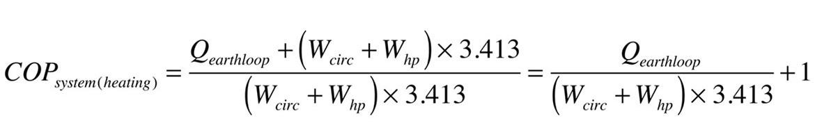
We also discussed the concept of system COP which includes the electrical input power to both the heat pump and earth circulator. System COP is a more relevant metric of geothermal heat pump performance since the owner is paying for the electrical energy to operate the heat pump and the circulator, and their operation is always simultaneous. System COP, in heating mode, was defined as follows:

Formula 1

where:

COP_{system(heating)} = Coefficient of Performance of heat pump + circulator as a system.

Q_earthloop = heat delivery rate of earth loop to heat pump (Btu/h).

W_circ = electrical input wattage to earth loop circulator (watts).

W_HP = electrical input wattage to heat pump (watts).

3.413 = conversion factor from watts to Btu/h.

We concluded last month’s column with the concept of a control that would continually vary the earth loop flow rate over small increments while searching for conditions that optimized system COP. We called the concept maximum COP tracking.

Step by step

Here’s the concept for a control algorithm for maximum COP tracking that is applied in heating mode.

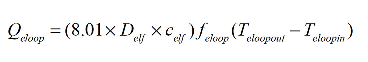
1. Measure the rate of heat transfer from the earth loop using temperature change, flow rate and fluid properties (e.g., density and specific heat) measured at the average temperature of the earth loop. These parameters would then be combined using Formula 1.

Formula 1:

Where:

Q_eloop = rate of heat delivery from earth loop (Btu/h).

8.01 = units conversion constant.

D_elf = density of earth loop fluid at average loop temperature(lb/ft3).

c_elf = specific heat of earth loop fluid at average loop temperature (Btu/lb/°F).

f_elt = flow rate through earth loop (gpm).

T_eloopout = temperature of fluid returning from earth loop (°F).

T_eloopin = temperature of fluid entering earth loop (°F).

F_eloop = flow rate in earth loop (gpm).

2. Measure the total input wattage to the heat pump (Whp), and the earth loop circulator (Wcirc). This may be possible using a single power transducer for systems that power the earth loop circulator from the heat pump.

3. The system COP in heating mode can be calculated as Formula 2:

Formula 2:

FIGURE 1

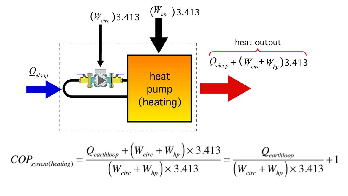
This assumes that the power to operate the circulator is ultimately converted to heat and dissipated into heated space.

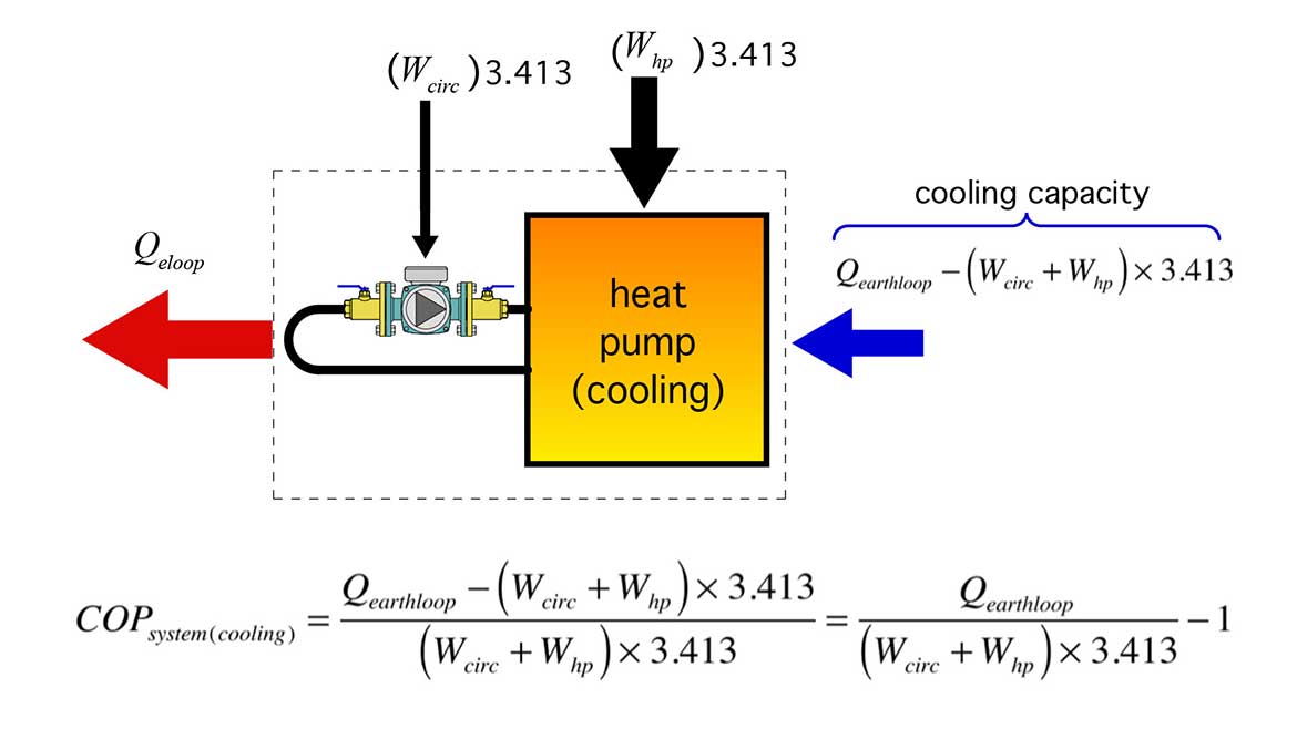
The system COP in cooling mode, is the cooling output divided by the total electrical input to the heat pump and circulator. It can be calculated using Formula 3:

Formula 3:

FIGURE 2

4. When heat pump first starts in heating mode, operate earth loop circulator at full speed.

5. Monitor the incoming loop temperature for a few minutes until it is relatively stable.

6. Calculate the system COP based on Figure 1.

7. Increment the loop circulator speed down slightly, and allow the incoming loop temperature to stabilize, then recalculate the system COP. If the new system COP is higher than before, operate at this speed.

8. Repeat incremental reductions of earth loop circulator speed, each time allowing the entering earth loop temperature to stabilize, and then calculate the new system COP. If a drop in system COP occurs upon a drop in circulator speed, increment circulator speed upward, stabilize and recalculate system COP. Move the pump speed in the direction that continually maximizes the system COP.

This feedback control loop would likely be operated based on PID (proportional, integral, derivative) algorithm. It could be self-tuning to adapt to system with larger thermal mass.

A similar algorithm would be used to adjust the earth loop circulator speed when the system operates in cooling mode. The math would be based on Figure 2.

Abundant sensors

This concept is more viable today than in the past, largely due to increasing availability of relatively inexpensive flow rate and electrical power transducers.

Some currently available flow sensors are based on vortex shedding while others use turbines. Most output a pulse signal, in some cases several hundred pulses per gallon of passing flow. An example of a 1.5-inch pipe size flow sensor is shown in Figure 3.

FIGURE 3

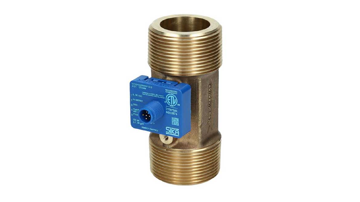
The flow rate measurement would be combined with earth loop inlet and outlet temperature measured with thermocouples or thermistors that can accurately measure temperature to within 0.1° F.

The controller (or building automation system) would store mathematical curves for the density and specific heat of the earth loop fluid as a function of the average loop temperature. That information, combined with flow and temperature difference allows the controller to process Formula 1 to determine the rate at which the earth loop is delivering heat to the heat pump.

The electrical power input for the heat pump and earth loop circulator can be measured by a power transducer. If the circulator is powered through the heat pump — typical of small single-phase heat pumps — a single power transducer will suffice. If the circulator is powered through a different circuit, a second power transducer is required. Figure 4 shows an example of a small single-phase power transducer.

FIGURE 4

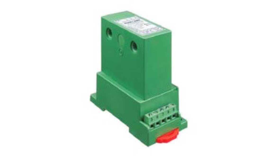
The power transducer used should create an output signal proportional to real power (a.k.a. “active” power). Most power transducers in this range can output a 0-10 VDC, 4-20 ma, RS485 signal that’s proportional to power.

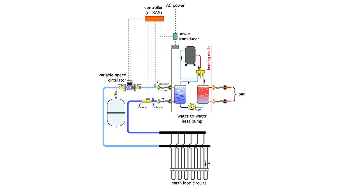
Figure 5 shows the placement of the sensors and transducers.

FIGURE 5

Small and low-cost microcomputers such as the Arduino or Raspberry PI could likely be configured and programmed to handle all the sensor inputs, calculations, and outputs necessary to provide maximum COP tracking. On larger projects, where building automation systems are used, a few lines of custom code would likely provide the necessary calculations.

This method of control doesn’t necessarily seek to maintain turbulent flow. Instead, it seeks to optimize the ratio (e.g., system COP) that yields the greatest amount of useful heat (or cooling capacity) per unit of electrical energy supplied to the plant. If that happens to correspond to turbulent flow, fine. If not, that’s also fine.

Hopefully, this discussion will inspire further testing and produce development that helps optimize the system COP of ground source heat pumps.

As we close out 2023, I wish you and your families a blessed and joyous Christmas.