✕

The geothermal heat pump market has changed quite a bit since its early commercialization in the 1980s. Back then, all geothermal earth loops operated with fixed-speed circulators. Those circulators were typically sized to ensure that the flow through the earth loop circuits remained turbulent under the harshest expected conditions. That condition was based on the Reynolds number of the flow stream. According to the IGSHPA (International Ground Source Heat Pump Association) Design and Installation Guide, Reynolds numbers need to be at least 2500 to ensure turbulent flow in earth loops.

A quick review

If you’ve dealt with pipe sizing in HVAC systems chances are you’re familiar with the concept of Reynolds number. It’s essentially a ratio of the inertial forces acting on a fluid divided by the viscous forces working on that same fluid. When inertial forces dominate the flow will be turbulent. When viscous forces dominate the flow will be laminar.

The Reynolds number can be calculated using Formula 1.

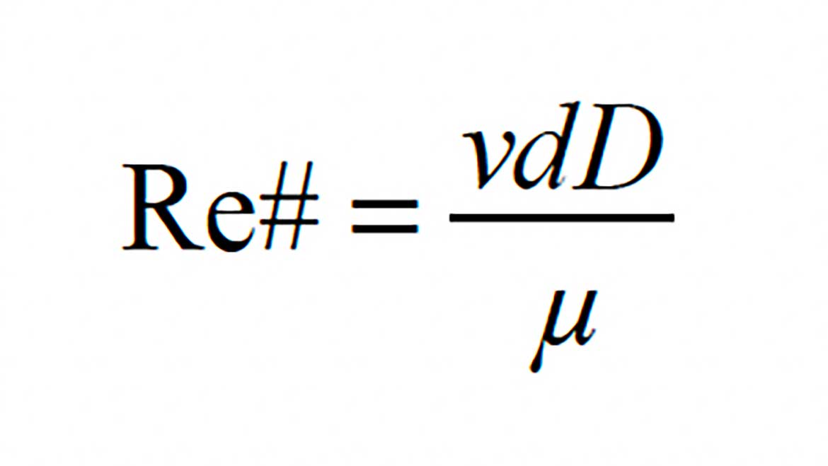
where:

v = average flow velocity of the fluid (ft/sec)
 d = internal diameter of pipe (ft)
 D = fluid’s density (lb/ft³)
µ = fluid’s dynamic viscosity (lb/ft/sec)

The Reynolds number is always a unitless number. All the units on the parameters used to calculate it must mathematically cancel out when combined in Formula 1. If they don’t, the calculation is missing one or more necessary unit conversion factors. Any calculated value for a Reynolds number, that is not unitless, is invalid.

Here’s an example: Determine the Reynolds number for a 20% solution of propylene glycol and water, passing through a 1-inch DR-11 (ratio of pipe OD to wall thickness) high-density polyethylene (HDPE) pipe, at a flow rate of 5 gpm. Assume the temperature of the solution is 30° F.

Before applying Formula 1, several values must be calculated or looked up. First, it is necessary to determine the density and dynamic viscosity of the 20% solution of propylene glycol at its temperature of 30° F. These values can be referenced in tables or software provided by the fluid manufacturer. When referencing viscosity, be sure the units are the same as those listed for Formula 1 (e.g., lb/ft/sec). If they are not, first convert the stated viscosity into units to lb/ft/sec before using Formula 1.

One manufacturer’s reference information lists the following for a 20% solution of inhibited propylene glycol.

D = 64.14 lb/ft³

Viscosity = µ = 4.23 cps = 4.23 centipoise.

The referenced viscosity can be converted to the necessary units as follows:

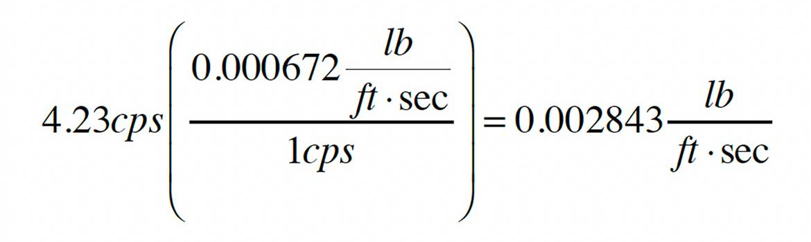
Thus, µ = 0.002843 lb/ft/sec

The average flow velocity can be found using Formula 2, and the exact inside diameter of the 1-inch DR-11 HDPE pipe.

Formula 2:

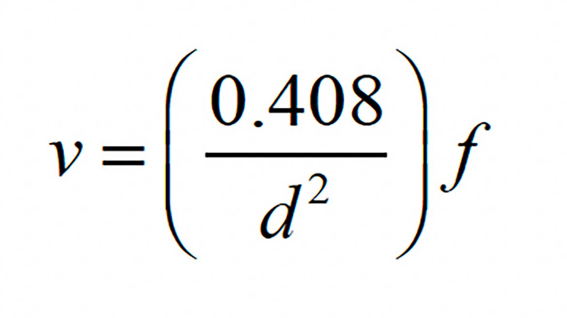
Where:

v = average flow velocity (ft/sec)
 d = exact inside diameter of tube (Inch)
 f = flow rate (gpm)

A 1-inch DR-11 HDPE pipe has an internal diameter of 1.076 inches. Putting this information into Formula 2 yields the average flow velocity:

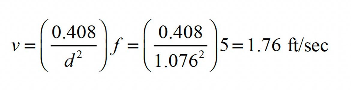
The gathered numbers can now be entered into Formula 1 to obtain the Reynolds number.

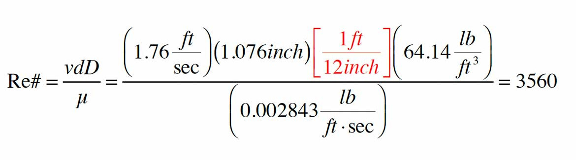
The Reynolds number of 3,560 is well above the minimum value of 2,500, and thus the flow will be turbulent under these conditions. Remember, the Reynolds number must always be a unitless value. The best way to ensure that a valid Reynolds number is being calculated is to include the units along with the numerical values for all the input data, and then make sure the units mathematically cancel prior to running the numbers through a calculator.

The higher the Reynolds number, the more turbulent the flow. Turbulence increases the convection coefficient for heat transfer between the fluid and inside surface of the tube. For a 20% solution of propylene glycol at 25° F, the theoretical convective heat transfer coefficient associated with mildly turbulent flow is about 14 times higher than for laminar flow. From the standpoint of heat transfer only, the higher the Reynolds number, the better the heat transfer.

However, higher flow rates and increased turbulence also mean higher head loss and thus more pumping power.

Conservative design practice

The generally accepted approach for sizing earth loops is to establish a minimum flow rate that ensures turbulent flow. That flow rate depends on the density and dynamic viscosity of the fluid at the lowest expect temperature within the earth loop.

Horizontal earth loops in Northern climates can create fluid temperatures in the range of 20-30 ºF by the end of a typical heating season. The lesser the amount of tubing used, relative to the capacity of the heat pump, the lower the loop temperature is likely to be.

The dynamic viscosity of propylene glycol solutions increases rapidly at low temperatures, as shown in Figure 1. This fluid property is typically the limiting factor in the minimum flow rate calculation.

Figure 1

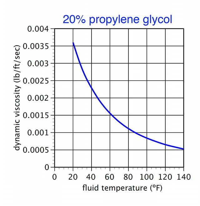
Figure 2 shows the effects of glycol concentration and fluid temperature on the minimum flow rate to ensure turbulent flow in a 1.25-inch nominal DR-11 HDPE pipe.

Figure 2

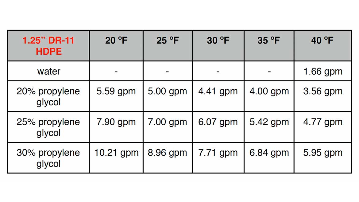
At a fluid temperature of 30° F, increasing the propylene glycol concentration from 20% to 30% increases the required minimum flow rate for turbulence by 75%. Lowering the fluid temperature from 30° to 20° F increases the required minimum flow rate by about 27%.

Similar tables are available for other pipe sizes and antifreeze fluids. A suggested reference is Ground Source Heat pump Residential and Light Commercial Design & Installation Guide, published by the IGSHPA.

Keep in mind that the required minimum flow rate for turbulence is a design condition. There will be many hours when the fluid temperature is higher, and thus the viscosity will be lower and the Reynolds number will increase.

Leveraging an opportunity

This significant variation in viscosity and its effect on minimum flow rate implies an opportunity for variable speed pumping for the earth loop. Flow rates could be lowered at higher fluid temperatures while still maintaining turbulent flow.

In theory, it would be possible to build (or program) a controller that could continually calculate Reynolds number, and provide a speed control signal to the earth loop circulator so that the Reynolds number is maintained above 2500. Unfortunately, there are some practical considerations that would make this approach questionable.

First, there would have to be absolute certainty on the glycol concentration in the system fluid, along with assurance that manufacturer’s data for dynamic viscosity and density are accurate.

Second, the temperature of the fluid used to calculate density and dynamic viscosity would have to be based on the coldest location in the earth loop, and very accurately measured.

This would make for an interesting experiment, but, in my opinion, remains a bit risky to implement until and unless such experiments prove that it’s reliable.

Another approach to varying the flow rate through an earth loop is based on what I call “Maximum COP tracking.” This approach measures the thermal output from the heat pump and the electrical power supplied to the heat pump and earth loop circulator. The “system COP” of the heat pump and its associated earth loop circulator, in heating mode, can be expressed as Formula 3.

Formula 3

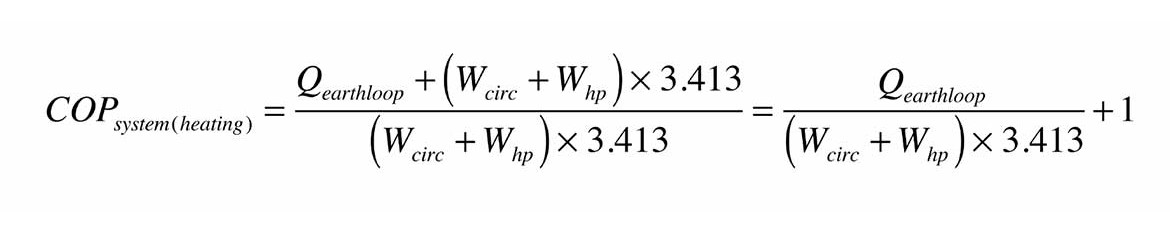
where:

COP_{system(heating)} = Coefficient of Performance of heat pump + circulator as a system

Q_earthloop = heat delivery rate of earth loop to heat pump (Btu/h)

W_circ = electrical input wattage to earth loop circulator (watts)

W_HP = electrical input wattage to heat pump (watts)

3.413 = conversion factor from watts to Btu/h

The goal is to keep the system COP as high a possible as the operating conditions of the heat pump change. The logic behind maximum COP tracking is to continually look for an earth loop flow rate that improves the system COP. It’s done by starting the earth loop circulator at full speed, measuring electrical input power to the heat pump and circulator, measuring the heat transfer rate from the earth loop, then using these measurements to calculate the system COP at this condition.

Next, the flow rate is incremented down slightly, the system is allowed to stabilize briefly, and the system COP is again calculated. If it increases, the flow rate will again be incremented down slightly and the process repeated. If the system is operating at some nominal flow rate, and the next decrease in flow rate causes the system COP to decrease the flow rate will be incremented up slightly, and the process repeated.

I’ll lay it out for you in more detail in next month’s Heating with Renewable Energy column.