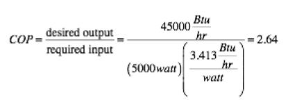
The measure of a heat pump’s heating performance is called coefficient of performance (COP). It’s the ratio of useful heat output divided by required energy input, where both the output and input are expressed in the same physical units.

For example, if an air-to-water heat pump delivers 45,000 Btu/h of heat output to a stream of water, and has a power input of 5,000 Watts, its COP, under those specific operating conditions can be calculated as follows:

The higher the COP, the greater the desired output is relative to the required input. Thus, higher COPs always are preferred, all other things being equal.

Although higher COPs result in lower electrical energy consumption, it’s important to realize that the person paying the bill for heating a building doesn’t pay for COP. They are paying for the Kilowatt•hours (kWh) of electrical energy necessary to run the heat pump and any other equipment, such as circulators, associated with running the heat pump. This is an important distinction and one that’s often misinterpreted when evaluating the merit of one heat pump versus another.

So, how is one supposed to evaluate various heat pump options with differing COP information and different installed cost? 

Start by understanding that COP can be calculated in several ways. The two most common ways COPs are expressed are:

1. As an instantaneous performance index; and
2. As a seasonal average value.

The instantaneous COP of any heat pump is strongly dependent upon all of the following:

1. The temperature of the material from which low temperature heat is being absorbed;
2. The temperature of the material to which higher temperature heat is being released;
3. The flow rate of the material supplying the low temperature heat (e.g., air or water) across the heat pump’s condenser; and
4. The flow rate of the material absorbing the higher temperature heat (e.g., air or water) across the heat pump’s condenser.

Most heat pump manufacturers list the COPs of their heat pumps under specific combinations of the above conditions. Those conditions usually are referenced to some industry standard, which should make it easier to make apples-to-apples comparisons.

It’s also important to realize that if any of these four operating conditions change, so will the COP and heating capacity of the heat pump. Under favorable operating conditions, it’s possible for just about any heat pump to have impressive COP values. Unfortunately, those favorable conditions, which represent a “snapshot” of performance, don’t exist over an entire season (if at all).

Conditions change

When evaluating seasonal heating cost it’s important to use a COP that reflects the wide range of operating conditions the heat pump will experience over an entire heating season.  These seasonal average COP values are not published by heat pump manufacturers because they don’t know what conditions the unit will operate under.

Still, it’s possible to simulate those conditions using software that factors in either hourly data for outdoor temperature or bin temperature data, and in the case of geothermal heat pumps, algorithms for heat transfer for specified earth loop configurations. Software simulations also have to account for the variations in the heat pump’s heating capacity and COP under all these conditions. In some cases the simulation also may have to adjust for time-of-use electrical rates. Such rates, where available, can significantly impact the operating cost for heat pumps that spend much of their total run time under lower off-peak rates.

The result of such a simulation would be a reasonable estimate of the heat pump’s heating season average COP, and that would be the performance index appropriate for making operating cost comparisons.

One vs. another

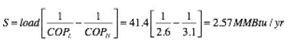
The annual savings in heating energy between two heat pumps with different heating season average COPs can be estimated using Formula 1.

Where:

S = savings in seasonal heating energy (MMBtu*)

load = total annual heating energy required for the building (MMBtu*)

COPL = seasonal average COP of heat pump having the lower of the two COPs

COPH = seasonal average COP of heat pump having the higher of the two COPs

Here’s an example: A house has a design heating load of 30,000 Btu/h when the outdoor temperature is 0° F, and the indoor temperature is 70°. The house is located in Syracuse, N.Y., with 6,720 annual heating °F•days. The estimated annual space heating energy use is 41.4 MMBtu. Assume that one heat pump option has a heating season average COP of 3.1. The other heat pump has a heating season average COP of 2.6. Putting these values into Formula 1 yields:

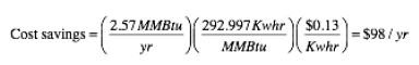
The cost savings associated with an energy savings of 2.57 MMBtu/h

depends on the cost of electricity. For example, if electricity sells at a flat rate of $0.13/kWh, the cost savings would be:

The COPH of 3.1 is an estimated average heating season COP for a geothermal water-to-water heat pump, supplied from a closed-loop vertical earth loop, in the central N.Y. area.  This COP includes an allowance for the electrical energy used by the earth loop circulator(s) in addition to the electrical energy used by the heat pump’s compressor. The assumed heating distribution system was a low-temperature radiant panel requiring a supply water temperature of 110° at design load.

The seasonal average COPL = 2.6 is an estimated average heating season COP for a low ambient air-to-water heat pump operating in the same location and connected to the same distribution system.

The question this calculation leads to is: Can an annual savings of $98 justify the higher installed cost of the geothermal heat pump?

There’s no simple answer. It depends on the installed cost of both system options, available subsidies, any cost escalation in electrical energy, the assumed life of both systems, and any maintenance cost associated with either system over that life.

However, even without specific numbers on the above costs, there’s still an important takeaway, and it’s based on Formula 1: 

The savings associated with a heat pump having the higher seasonal COP, relative to one with a lower seasonal COP is directly proportional to the building’s annual heating energy requirement.

Cut the building’s heating energy usage in half and the savings are cut in half. Therefore, savings associated with a heat pump system yielding a “phenomenal” average heating season COP of 4.0 versus one with a more “mediocre” average heating season COP of say 2.5, in a building with a design load of only 18,000 Btu/h, in Syracuse would be:

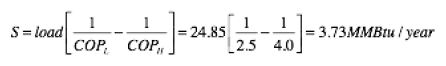
At a going rate of $0.13 per kWh, the annual savings would be about $142 per year.  That’s about 24% of what many households spend for a year of internet service at $50 per month.

I’m not against high efficiency heating systems. Quite the contrary, our industry should always be striving for improvements. But mass markets for such systems will only develop and sustain themselves when the economic case is justified.

When the savings are less than what many families spend on designer coffee it’s a hard case to make. It’s something to think about when contemplating a very high performance, but very pricey heating systems for low-energy buildings.

* 1 MMBtu = 1,000,000 Btu

To read Siegenthaler’s article “Comparing COPs” in pdf form, please see here.