The classic way of estimating heating load in smaller, envelope-dominated buildings is to assume the rate of heat loss is proportional to the difference between the inside and outside temperature.

The “design” heating load is estimated based on an outdoor temperature that is close to the lowest outdoor temperature for the location based on long term weather records. That temperature is called the 97.5% design dry bulb temperature. The reason heating load is not based on the 100% lowest outdoor temperature is because such a condition is very “short-lived.” It might only exist for one hour during one of several consecutive years. Basing the design heating load on such an infrequent and extreme temperature would lead to significant oversizing of the building’s heat source, especially if the designer hedges their estimate by including a generous safety factor. Furthermore, most buildings have sufficient thermal mass to “coast” through a short duration extreme low temperature when and if it occurs, using equipment sized for 97.5% design dry bulb temperature.

The indoor temperature commonly assumed for estimating heating load in spaces intended for human occupancy with normal clothing and light activity is 70° F. 

Using these design conditions, a strictly proportional relationship between heating load and inside/outside temperature difference would make the heating load zero when the outdoor temperature is 70° or higher.  It would also imply a small heating load exists if the outdoor temperature were to drop to 69°.  That small heating load would mathematically double if the outdoor temperature dropped to 68° and the indoor temperature was to remain at 70°. 

The owners of homes built over the last 40 years, as well as occupants of other small envelope-dominated buildings, know their heating systems don’t need to operate to maintain 70° inside temperature when the outdoor temperature is 69° or 68°.  The heating systems in most modern structures don’t need to add heat to interior spaces until the outdoor temperature drops well into the 50s, and in some cases even into the 40s.

Heat from modern living  

So why does simple mathematical theory imply that a heating load exists, yet experience shows that the heating system in many buildings does not need to operate under such conditions.

The answer in based on internal heat gains. The heat generated by sunlight through windows, operating appliances, computers, entertainment equipment, lights, cooking, bathing, standby heat loss from water heaters, all those little black box transformers and occupants can easily maintain a building at or above 70° when the outdoor temperature is significantly lower than 70°.

So how low can the outdoor temperature get before internal heat gains can no longer meet the heating load? That temperature is called the “balance point” temperature of the building. It can be estimated based on the interior temperature that needs to be maintained, the total rate of internal heat gain and the heat loss characteristic of the building. These parameters come together as Formula 1.

Where:
Tbalance = balance point temperature for building (°F)
Tin = interior temperature of building (°F)
Qgain = rate of interior heat gain (Btu/h)
UAbldg = heat loss coefficient of building (Btu/h/°F)

Here’s an example of how this formula can be used: Assume a building has a design heat loss of 24,000 Btu/h when the inside temperature is 70°, and the outdoor design dry bulb temperature is -2°.  The building is heated by a gas-fired boiler, and thus doesn’t intentionally use electricity to generate heat. The building and its occupants create a typical monthly electrical energy consumption of 1100 kWh during the heating season months. Further assume that 80% of the daily electrical usage occurs between 6 a.m. and 10 p.m. Estimate the balance point temperature based on this information.
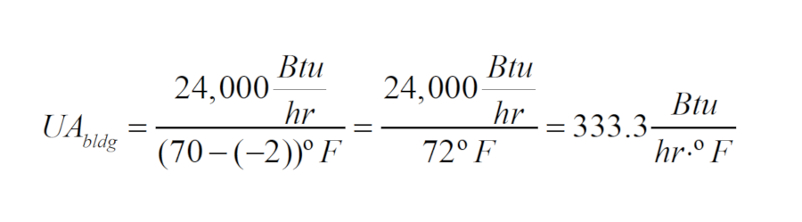
Let’s start with the building heat loss information. The value for UAbldg is just the design heat loss rate divided by the corresponding difference between inside and outside temperature.

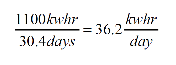
An average month has 365/12 = 30.4 days. Thus, the daily average electrical usage is:

The hourly average electrical consumption between 6 a.m. and 10 p.m. — assuming this period represents 80% of the total daily electrical energy use, would be:

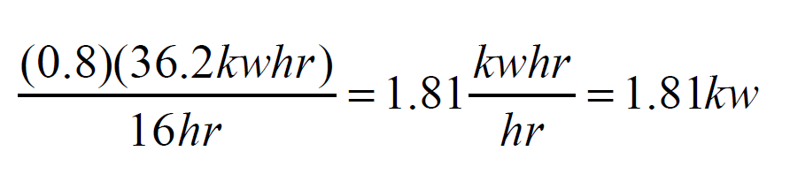
Notice the units of hour cancel out in the top and bottom of this fraction to give an average rate of internal heat gain equal to 1.81 kw.
This rate in kilowatts can be converted to a rate in Btu/h:

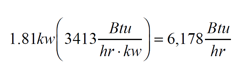
That’s a significant rate of heat input. In this example, it’s over one quarter of the building’s design heating load. It’s also just based on electrical usage. There could also be solar heat gain if the building has southern facing windows and a reasonable southern exposure.  

People heat  

It’s also prudent to include some contribution to internal heat gain from occupants. Let’s assume the equivalent of two adults engaged in light activity during the hours between 6 a.m. to 10 p.m. Each person would contribute another 512 Btu/h to the internal heat gains. So, assuming negligible solar gain, the total rate of internal heat generation in this example is:
 

There’s now sufficient information to calculate a balance point temperature using Formula 1:

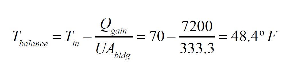
The implication of this result, based on all the assumed conditions, is this building would not require any heat input from it’s heating system until the outdoor temperature dropped below approximately 48°.

Nullifying affect  

I wanted to see how the balance point temperature of a building might affect the seasonal performance in an air-to-water heat pump.  

In last month’s Heating with Renewable Energy column, I shared the results of a spreadsheet I developed which used bin temperature data for Syracuse, New York, along with performance information for a specific air-to-water heat pump installed in a well-insulated house (UAbldg=450 Btu/h/°F) to estimate the heat pump’s seasonal average coefficient of performance (COP). In addition to space heating, the system I modeled included an assumed domestic water heating load of 60 gallons per day, heated from 50° to 120°. Some of this DHW load was handled by heat supplied by the heat pump, and absorbed from a buffer tank through a heat exchanger. The temperature of the buffer tank was based on outdoor reset control. The supplemental heat required to fully heat the domestic water to 120° was provided by electric resistance heating.  

The simulation yielded an estimated seasonal average COP of 2.85. This meant that every kWh of electrical energy suppled to operate the system transferred 2.85 kWh of useful heating energy to the loads. 

The initial runs of these simulations did not include the effect of internal heat gain, and thus simulated a small heating load at relatively high outdoor temperatures in the range of 50° to 65°. These outdoor temperatures, in combination with a low supply water temperature to the heat emitters based on outdoor reset allows the heat pump to operate at high COP, and thus tends to push the seasonal average higher. To prevent what I consider unrealistic heat pump performance, I limited the maximum simulated COP to 4.5 regardless of conditions that theoretically could have produced higher COPs.

To see how internal heat gains affected the simulation, I assumed the house would have a balance point temperature around 48°, and thus did not generate any heating load for the hours when the outdoor temperature was at or above 48°. Assuming all other conditions remained the same, the seasonal average COP decreased from 2.85 to 2.65, a drop of about 7%.

It’s worth mentioning that no solar heat gains were included. A house with good southern exposure and reasonable amount of southern side windows could have a balance point temperature much lower than 48° during the day. This would further decrease the heating load and further limit air-to-water heat pump operation under what would otherwise be quite favorable conditions.

Still, a seasonal average COP of 2.65 in a cold climate application is reasonably good performance. If electricity cost $0.12/kWh, this average COP would provide heating energy at an average cost of $13.27 per MMBtu. In central New York, this compares to $12.62 per MMBtu for natural gas in a 92% efficient heating appliance. In rural upstate New York, where natural gas isn’t available, it compares to $29.13 per MMBtu for heat derived from propane combusted at 92% average efficiency. 

The take away is internal heat gains will reduce heating loads, especially “light” heating loads at the beginning and end of the heating season. This will “nullify” some of what would otherwise be very favorable operating conditions for an air-to-water heat pump. However, the decrease in seasonal performance is not, in my opinion, a deal breaker. The seasonal average performance of a modern cold-climate air-to-water heat pump can still deliver heating energy at prices that are currently competitive with natural gas, and far lower than propane, fuel oil,or electric resistance heating in an upstate New York location.