Issue: 1/06
I often get involved with discussions of the surface temperature of a heated floor. Perhaps it's in the context of not allowing the slab to exceed the recommended 85°F surface temperature in situations of prolonged foot contact with the floor. Other times, it's a discussion of "striping"
Painting by Numbers
Not being much of an artist, I occasionally resort to mathematically generated scenes using a technique called finite element analysis (FEA). This is a technique that engineers who suffered through the complex theoretical mathematics of two-dimensional heat conduction can really appreciate. It approximates the solution of partial differential equations that govern such heat transfer. This is done by breaking the cross-section of the material assembly being analyzed into hundreds or even thousands of small adjacent pieces (e.g., finite elements), and calculating heat flows in and out of each one of them.
For steady state heat transfer, the heat flowing into and out of each of these elements must be equal. The temperature of each element will settle to a value that makes this possible. The balanced heat transfer is described by hundreds or thousands of simultaneous linear equations, which would be virtually impossible to solve without the number crunching power of a computer. Thirty years ago, such a situation required a mainframe computer and lots of computing time. Today, the cheapest department store computer can do these calculations in a couple of seconds. That solution is a temperature value for every element in the cross-section.
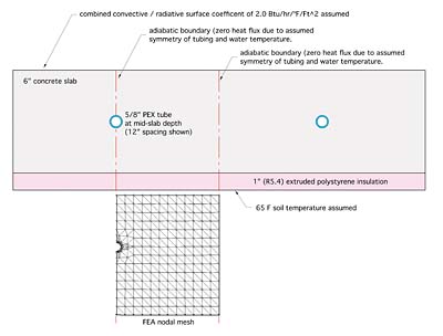
Notice the adiabatic boundaries in the slab cross-section. These are boundaries across which no heat transfer is allowed due to symmetry of tubing placement and the assumption that water in the adjacent tubing is at the same temperature.
Arguably, the latter assumption is slightly flawed in that water temperature continuously decreased along the length of the circuit. However, in a system with serpentine tubing placement, it's still a reasonable approximation, and one that's necessary to develop an FEA model without resorting to 3D complexities.

The PEX tube is modeled as a multi-sided polygon that approximates the round shape in a manner that simplifies FEA mesh creation. The tube wall is shown within the blue outline in Figure 2. The number of nodes in the vicinity of the tube is higher to better approximate the higher heat flux in this region of the cross-section.
The Big Picture
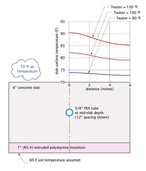
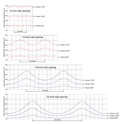
FEA models were created and run for a 6-inch thick concrete slab with tube spacing of 6, 12, 18, and 24 inches. For each tube spacing, the model was run for water temperatures of 80°F, 100°F, and 120°F. The surface temperature profiles based on the output of these models are shown in Figure 5.
It's also evident that the area under the curves decreases as the water temperature is lowered. This area is proportional to the heat output from the surface of the slab.
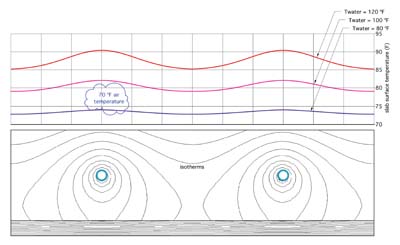
Figure 6 is a composite showing the surface temperature of all four tube spacings and three water temperatures. In each case, the surface temperature profile exists from the center of the tube to a point halfway to the adjacent tube.
What About Heat Output?
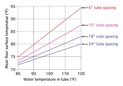
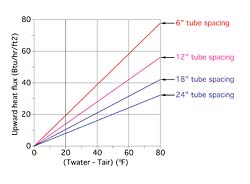
Surface temperature profiles are interesting to look at, but designers need to know how they translate into heat output. Data from the FEA models was analyzed to attain average surface temperatures. This in turn was used along with an assumed radiative/convective surface heat transfer coefficient (2.0 Btu/hr/°F/ft2) to generate the upward heat flux graph shown in Figure 7.
This graph shows upward heat flux as a function of the difference between the water temperature in the circuit and the room air temperature. Think of the water temperature used to calculate this difference as a value at a given location along the circuit. Obviously this temperature is highest at the beginning of the circuit and drops as water flows along the circuit. If these temperatures are known, or can be estimated, one can compare heat flux at the beginning and end of the circuit.