
I’ve written several “Heating with Renewable Energy” columns covering the benefits of combining modern hydronics technology with modern air-to-water heat pumps.
One of the two most salient points stated in all those columns was that the heating output of any air-source heat pump decreases with increasing water temperature and/or decreasing outdoor temperature. The other was that the heat pump’s coefficient of performance (COP) always increases as the temperature at which the hydronic distribution system operates decreases.
The concept given in that last sentence is a “qualitative” statement, one that usually leads designers to ponder a follow-up “quantitative” question: How much does the heat pump’s COP change over a range of system operating temperatures?
If the change is small, it may not justify additional investment in the heat emitters to allow low-temperature operation. On the other hand, if there’s a significant change in COP with water temperature, it could have profound implications for the system’s life cycle operating cost.
Number crunching
A recent project I’ve been working on was designed to put numbers to the qualitative concept regarding COP.
My colleague and top-notch engineer, Mario Restive, worked with me to develop a detailed simulation software for hydronic systems supplied from an air-to-water heat. It combines weather data files for 14 locations in New York state, with performance curves for several air-to-water heat pumps. It also includes building heating load models, cooling load models, corrections for internal heat gains, heat pump defrosting, circulator energy and outdoor reset lines representing a wide range of heat emitters. It also has the ability to include a specified domestic water heating load.
The simulation software allows the heat pump to provide heat to loads at water temperatures up to 130° F. If higher water temperatures are required, such as in a legacy hydronic baseboard system on a cold upstate New York winter day, the model calculates how much auxiliary energy is associated with those higher temperature requirements.
Reasonable results
The number crunching taking place in the simulation software produces several outputs associated with the system’s seasonal thermal performance, as well as its operating and owning cost.
Two of the thermal results are: The heat pump’s annual average COP and the percent of the annual space heating plus domestic water heating energy supplied by the heat pump.
I ran the software for a representative case with the following assumptions:
Weather data location: Plattsburg, New York (way up there just below Canadian border, and averaging 8,000+ °F•days)
Heat pump: Nominal 4-ton rated, low ambient unit with a vapor injected/single speed compressor)
Building envelope: Design heating load of 36,000 Btu/h at -9° F outdoor, and 70° F indoor temperatures
Average internal gain: 2 kw (6826 Btu/h)
Domestic water heating load (when used): 60 gallons per day heated from 50° to 120° F.
Supply water temperature required at design load: 100, 120, 140, 160, 180° F
Full outdoor reset of supply water temperature.
The table in Figure 1 shows the heat pump’s annual average COP, and the percentage of the building’s space heating load covered by the air-to-water heat pump. No DHW load was assumed for the simulations represented in Figure 1.
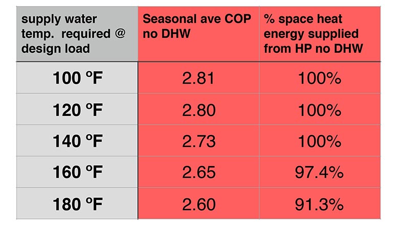
What the numbers mean
The seasonal average COP definitely goes down as the design load supply water temperature goes up. Still, even when the distribution system needs 180° F at design load, the use of outdoor reset allows the heat pump to attain a seasonal average COP of 2.6. That’s reasonably good for an air source heat pump in a cold climate application.
The size of the heat pump (nominal 48,000 Btu/h), relative to the building’s design heating load (36,000 Btu/h), allows it to cover all of the space heating energy in systems with design load supply water temperatures of 140° F or less. The percent of load drops off, as expected, in systems requiring water temperatures higher than the heat pump can provide. However, even in the high temperature system, the heat pump is covering about 91% of the buildings total space heating energy requirement.
Add in DHW
Unlike space heating, domestic water heating is a year round load. As such, it allows the air-to-water heat pump to operate at high COP during the “non-heating” months — typically May through September. A DHW temperature lift of 50-120° F is also well within the operating range of the heat pump.
Our simulation includes control logic that allowed the heat pump to operate at a setpoint temperature of 5° F above the temperature to which domestic water was being heated — but in no case higher than 130° F. This control logic was used for times when no space heating load was present. It allows the heat pump to provide a higher percentage (sometimes even 100%) of the DHW load during the non-heating months. The 5° F difference between the DHW setpoint and the upper temperature limit of the heat pump, was to account for the temperature drop across a generously-sized heat exchanger separating system water from domestic water.
When a domestic water load of 60 gallons per day, heated from 50 to 120° F, was included in the simulation, the heat pump’s annual COPs increased slightly, as seen in the blue shaded area of Figure 2.
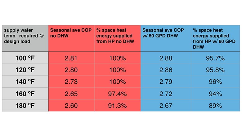
Since the heat pump was assumed to operate with outdoor reset during the heating season, it could not supply the upper temperature end of the domestic water heating “lift”. This shows up as a slight decrease in the % of the total load (space heating + DHW) supplied by the heat pump. Any heat added to domestic water, but not supplied by the heat pump, was assumed to be supplied by electric resistance heat.
Warmer venues
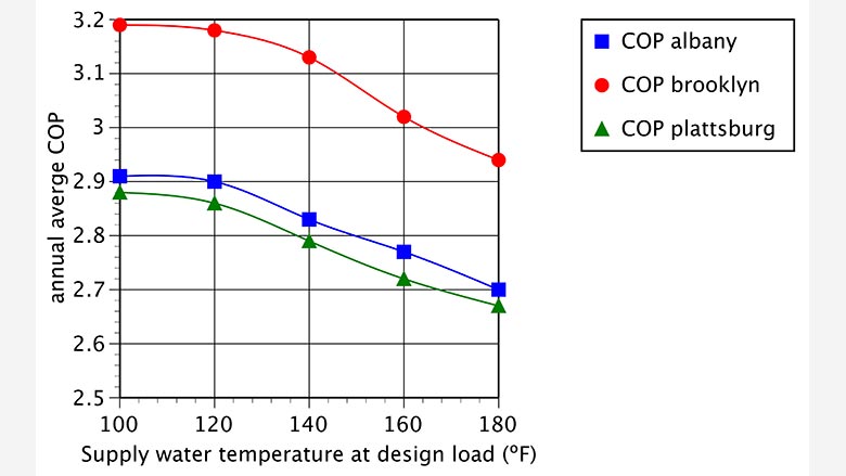
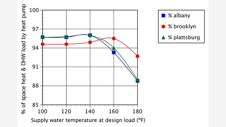
I also ran simulations for warmer New York state climates, specifically Albany and Brooklyn. The design space heating load of 36,000 Btu/h based on the Plattsburg location was adjusted for these other locations so that the same building was simulated in all three locations. A domestic water heating load of 60 gallons per day, heated from 50° to 120° F was also included in all three locations.
As expected, heat season performance increased as the number of degree days decreased. Figures 3 and 4 show the variation in annual COP and percentage of the heating load covered by the heat pump.
The “take aways”
Here’s a summary of what I believe these simulations are indicating.
- Although there’s a definite improvement in annual heating performance over the full range of design load supply water temperatures, that variation is quite small between 100° and 120° F. This suggests that hydronic distribution systems can be used at design load temperatures up to 120° F, without any significant compromise in annual heat pump performance.
- The heat pump’s contribution to the annual space heating plus DHW load drops as water temperature increases, but it still supplies the majority of the seasonal heating energy, even in a “legacy” hydronic system requiring 180° F water at design load. This supports the use of air-to-water heat pumps as a retrofit strategy for legacy hydronic heating systems, but also indicates that a supplement heat source (such as the system’s existing) boiler will be needed for the coldest winter days.
- The range of annual COPs achieved by the air-to-water heat pump used in these simulations was, in my opinion, relatively good. When an annual average COP of 2.75 is combined with the spring 2022 price of electricity in central New York, the cost of delivered heat on a $/MMBtu basis is less than half that of propane and fuel oil, (again based on spring 2022 pricing), and only marginally higher than that of natural gas.
It’s a simulation, not a guarantee
Simulations attempt to predict outcomes based on available data and computational methods. They are not “guarantees” of performance.
The simulations we used are based on relatively detailed models for physical objects such as the building, and the published performance information for a specific air-to-water heat pump. The simulations attempt to account for “real” effects such as how internal heat gain within a building affects its net heating load, or how defrosting reduces the energy available from the heat pump. The computations even count the wattage of the heat pump’s circulator, which is located inside the building, as a small contributor to heat input, and a small “adder” to building cooling load.
The results discussed are all specific cases with assumed equipment, a given building envelope, and other contributing factors. While the results suggest reasonable performance for the specific cases that were simulated, designers should not extrapolate the results to include “all” air-to-water heat pumps, in all buildings, in all climates.
Still, system design needs numbers to guide decisions. Simulations based on sound engineering principles and established performance models are far more practical and less costly than setting up real systems and monitoring their performance over multiple years. It’s a starting point that helps inform qualitative concepts with quantitative information.


