It all revolves around a very basic equation to determine velocity and rate of flow.
Editor’s Note: “Back to Basics” is a column that will run periodically in PM Engineer reviewing the basic principles of plumbing engineering.
Sizing a water piping system is relatively easy. The basic pipe flow equation is Q = VA. This equation can be converted to normal units of measure, as well as using the inside pipe diameter. The new equation would read:
Q = 2.448 V d2
Where:
Q = flow rate in gpm
V = velocity in ft/sec
d = diameter in inches
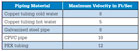
Table 1. Maximum Recommended Flow Velocities
Importance of Flow Velocity/Rate
When attempting to determine the appropriate pipe diameter for a water distribution system, one needs to know the velocity of flow and the flow rate. The velocity of flow is established by evaluating the performance of the piping material, the noise in the pipe, and the potential for elevated hydraulic shock.
Velocities of less than 12 feet per second tend to not create high levels of noise in the piping system. However, this high a velocity can result in higher intensities of hydraulic shock or water hammer. The system would have to be evaluated for protection from hydraulic shock.
Several piping-material manufacturers recommend maximum velocities of flow for plumbing water distribution systems. Table 1 lists the recommended maximum velocities.
When determining the pipe size, engineers often consider the anticipated length of time that the system will flow at the maximum velocity. If the maximum velocity is only anticipated for a short period of time, a velocity slightly higher than the listed velocities may be selected. When there is an anticipated continuous flow, a lower velocity is often selected.
With the velocity selected, the flow rate or “Q” must be determined. This is the hardest part of engineering a plumbing water distribution system. Plumbing fixtures are used on an intermittent basis. To determine the flow rate, the simultaneous use of the plumbing fixtures must be determined. This maximum flow rate is also known as the “peak demand.”
There are various methods for determining the peak demand of a water distribution system. The most popular method of determining peak demand is the Hunter Method. This method, using water supply fixture units, was developed by Dr. Roy Hunter in the early part of the 20th century. According to published reports by Dr. Hunter, he points out the inaccuracies of the method.
The Hunter Method assigns a water supply fixture unit to each fixture. This fixture unit value is a probability factor used to determine the total use of water within a given system. Hunter developed a curve that establishes the flow rate for any given water supply fixture unit value.
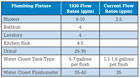
Table 2. Changing Flow Rates In Plumbing Fixtures
The Hunter Method originally assumed two types of buildings; one that used tank-type water closets and one that used flushometer-type water closets. The problem with this concept is that it does not account for the normal operation of a building. A football stadium will have a different demand on a water distribution system than an office building. Similarly, a large home with five bathrooms will have a different demand than an apartment with one bathroom.
The other concern with the original fixture unit design concept was the change in the use of water since the 1920s. All fixtures discharge a lower amount of water today. Table 2 points out the difference in flow rates from the 1920s to today.
When Hunter did his research, a typical home had one bathroom. Today, a typical home has 3, 4, 5 or 6 bathrooms. The size of a typical family is also less than when Hunter performed his studies.
These changes lead to a research project by the Stevens Institute of Technology to re-evaluate the Hunter Method. The project was considered somewhat controversial at the time, since many engineers wanted to do away with Hunter’s method and come up with a completely new design concept.
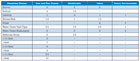
Table 3. Stevens Modified Fixture Unit Values
About the Stevens Method
The Stevens Method utilized the Hunter curve and simply adjusted the water supply fixture unit rates for each fixture. The new table lists values for four different categories of buildings. The categories include: one- and two-family dwellings, multifamily dwellings, high-use assembly buildings, and other buildings or commercial buildings. Some of the values of the new table are listed in Table 3.
The only Plumbing Code that completely includes the Stevens Method is the National Standard Plumbing Code. Both the International Plumbing Code and Uniform Plumbing Code include some of the provisions from the Stevens Method. It should be noted that all of the Plumbing Codes permit the water distribution system to be sized by accepted engineering practice. This would allow for the use of the Stevens Method.
The methods listed in Table 3 are for the total use of the water distribution system. When calculating the peak demand flow rate for the hot or cold water distribution system, the values in the table must be multiplied by 0.75.

Table 4. Flow Rates from Hunter Curve
To determine the size of the water distribution system, each fixture is assigned three values: the total water value fixture unit, the hot water fixture unit value, and the cold water fixture unit value. The values are added to determine the flow rate at any location in the piping system. The total fixture unit value is the number used for the pipe sizing upstream of the water heater.
When determining the flow rate using the Hunter or Stevens Method, the curve has two values - one listing is for flush tank water closets, the other is for flush valve. Table 4 lists some of the common flow rates on the Hunter’s curve.
Even with the modified Stevens Method, not all systems can be sized using this method. Like all sizing methods, there are limitations regarding high-end and low-end water distribution systems.
A good example would be a football stadium. Even the heavy-use assembly values will undersize the water distribution system for a football stadium. On the other extreme would be a row of lavatories that have aerators with a flow rate of 0.5 gpm. This method would oversize the flow rate for these fixtures. Any sizing method needs a common sense approach for establishing the flow rate in the piping system.
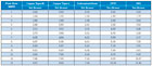
Table 5. Flow Rates and Velocities for 3/4-Inch Pipe
Once the flow rate is determined, the pipe size can be selected knowing the maximum design velocity and the diameter of the pipe. Table 5 lists the flow rates and velocities of flow for various piping materials that are 3/4 inch in diameter.
The table demonstrates the differences between the various piping materials. For a flow of 12 gpm, the velocity in the pipe ranges from a low of 7.22 feet per second for galvanized steel pipe, to a high of 10.57 feet per second for PEX tubing. This also demonstrates why the water distribution system must be sized base on the particular piping material that is to be installed. A general sizing for all piping materials would not produce the correct results.
Once the pipe size is selected, the pressure loss in the piping system must be evaluated (which is a separate topic). This is all a part of sizing a water distribution system.
