When people say that the “ends justify the means,” it is usually an excuse for screwing something up and shrugging their shoulders as if to say, “Oh well, I got the result I wanted and that’s all that matters.”  It reminds me of that impulse you have when you are a kid playing a practical joke that you know is probably a bad idea, but do it anyway because you want that thrill you feel after your plot, usually at someone else’s expense, has been executed. It’s all fun and games until someone gets hurt. After giving it some thought as it relates to engineering, I think I’ve come up with the answer to whether the “ends justify the means” and my answer would be… sometimes.

We as engineers are often guilty of taking things literally, and we can apply those skills to answer deep philosophical questions. If you’ve made it this far in life, chances are you’ve sat in a few classes and been graded on your performance. If you’re like me and went to school for engineering, you may have hoped and prayed that your class would be graded on a curve. Grading on a curve meant that if you got a test score of say 35% for example, you might not actually get a failing grade if the best score in the class was a 55%. 

Depending on how driven a student you were (or are) might reflect where your grades would land on the bell curve. As a refresher, a bell curve is a graphical representation of a “normal” distribution of data. Some data points will land on the far left of the curve, some on the far right, but most will land in the middle. The middle, which is the highest point of the bell curve, is known as the “mean,” defined as the mathematical average of two or more numbers. The width of the bell curve, or how far it spreads out at each end, is defined by a term known as “standard deviation.” Standard deviation is calculated by taking the square root of the variance, the distance from each number from the mean.

Let’s put this into context for something we all understand — toilet flush rates. For argument’s sake, I’m going to say that the average flush rate for a toilet is 1.44 gpf. This is the mathematical average of the LEED baseline flush rate of 1.6 and what is becoming an industry standard in some markets of 1.28. The variance in toilet flush rates is not too great, and if I were to envision a bell curve, it would be narrow and steep. The outliers on the high end might include some pre-1992 3.5 gpf boat anchors, clinic service sinks and a few toilets with broken flushometers from being kicked one too many times. On the low end, we would see some roadside composting toilets (which use zero water), 0.5 gpf airplane toilets, 1.0 gpf pressure assisted devices, or the lower flow dual flush units.

Here is a normal distribution of water closet flush rates with a standard deviation of 0.4 and a probability density of 1:

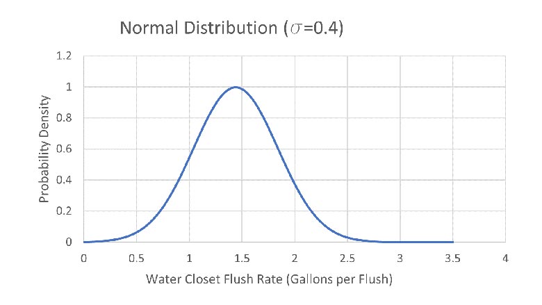
In order to achieve a probability density of 1, I input the standard deviation of 0.4. Standard deviation tells us how much observations of a data set differ from the mean. In order to get a more realistic picture of the normal distribution of installed water closets, I am going to decrease the standard deviation. Based on my professional experience as a plumbing engineer and personal experience using public water closets, I know that the standard deviation of water closets with various flush rates is much closer to 1.44 gpf. The below graph shows a normal distribution graph with a standard deviation of 0.2.

We can see by comparing the two distribution curves that water closet flush rates actually have a pretty high probability density. If we were to do a survey of all water closets throughout the United States, I have a hunch that the standard deviation is probably less than 0.2 and the probability density likely even higher than 2.0.

The other important factor to understand when discussing bell curves is called the scaling parameter. The first curve, with a standard deviation of 0.4 has a larger scaling parameter since the data fall wider to the left and right of the mean. You can see that it represents data as low as 0.5 gpf and as high as 2.5 gpf. The curve with a standard deviation of 0.2 falls closer in between 1 and 2 gpf.

In practicality, plumbing engineers all experience design challenges related to water closet flush rates. Sometimes we work for clients where the primary driver is water conservation or LEED points. We understand the technology that is available and the risks involved with specifying flush valves that fall too far to the left of the bell curve. I myself have been on projects with scorecards that use flush rates for flush valves that are not even available on the market. I’ve also been on projects where a higher flush rate is desirable for the maximum level of public safety. While we are limited by law on going above 1.6 gpf, I’ve actually heard engineers profess some type of Newtonian law of water conservation that “water is neither created nor destroyed,” so who cares about water conservation. While there may be some truth to the Law of Conservation of Mass, it does still cost money to use water and our clients do typically appreciate us being cognizant of that.

It should now be clear that there are times when the ends do justify the means. To justify is to show something to be right or reasonable. If we are specifying a water closet and the flush rate falls within the reasonable bounds of standard deviation, I would argue that the ends are justified because they are within the standard deviation of the mean. If we find ourselves falling outside the bounds of what is reasonable, we should do a double take — we might be going down a design or engineering path where the ends are just too far out and do not actually justify the means.