
Issue: 12/02
Although not specifically intended as heat emitters, the copper tubing connecting the components of many hydronic systems certainly does release heat to its surroundings. Sometimes designers disregard this heat output, assuming it's trivial relative to the heat released by the real heat emitters. Some might point out that if the tubing travels through heated space, the heat released is not really "lost" heat, it's heat delivered to the space by the tubing rather than the intended heat emitter. That may be true at times, but it still compromises an important and fundamental benefit of hydronic heat--the ability to deliver heat precisely when and where it's needed.
Heat released by the tubing connecting a water heater to a boiler is obviously not delivered to the intended load. The same is true for heat released by tubing to heat exchangers for pools, snowmelting and other loads.
To make informed decisions about tubing heat loss, the designer needs to know how much heat will be released under a given set of conditions. Chapter 22 of the 1989 ASHRAE Handbook of Fundamentals contains a table listing the heat output of bare copper tubing at different water temperatures, and when surrounded by 80 degrees F air. This temperature would be typical of piping in a mechanical room when heating equipment is operating. This table gives the designer "snap shots" of heat loss from bare copper tubing at specific temperature differences between the inside of the tube and the surrounding air.
If the designer needs to estimate the pipe's heat output at conditions not listed in the table, he/she could interpolate between the values. One might also plot the heat loss data, as shown in Figure 1.
To use this graph, one first determines the difference between the tube temperature and the surrounding air temperature. For example: If the inside temperature of a 1" copper tube is 150 degrees F, and the air temperature surrounding it is 50 degrees F, the temperature difference would be 150 - 50 = 100 degrees F. The tube's heat output, read from the graph, is approximately 56 Btu/hr/ft.
Continuous Temperature Drop
Although the ASHRAE data and Figure 1 give the heat output of one foot of bare copper tube at certain temperatures, they don't account for what happens when the water flows through the tube. Whenever heat is released from flowing water, its temperature drops in the downstream direction. The farther the water travels along the tube, the cooler it gets, and the lower the rate of heat output from the tube's surface becomes.If the tube is relatively short, or if the flow rate is high, the temperature drop from inlet to outlet will be small, perhaps even less than 1 degrees F. In such cases, the total heat output can be estimated by looking up the heat loss per foot in Figure 1 and multiplying this number by the tube's length.
Although this approach is simple and readily used in many situations, it somewhat overestimates the tube's total heat output, especially for longer tubing runs operating at low flow rates.
To correct for these situations, a more detailed procedure has been developed that accounts for differences in flow rate, surrounding air temperature, and tube length. This procedure gives more accurate results in situations where the tube's length in feet divided by its flow rate in gallons per minute is greater than 20.
The Math
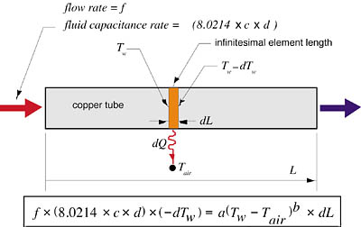
The analytical model for copper tube heat loss in circumstances not meeting the above criteria is given as Equations 2 and 3. Equation 2 is the solution to a differential equation describing the heat loss of an infinitesimal length of bare copper tubing of a given size surrounded by air, as shown in Figure 2.
The model was calibrated using the previously mentioned ASHRAE data fit to the function (see Equations 1, 2 and 3.)
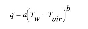
q' = heat output of a unit length of tubing (Btu/hr/ft)
Tw = temperature of fluid in pipe (degrees F)
Tair = temperature of air surrounding pipe (degrees F)
a, b = constants determined from a curve fitting procedure
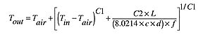
Tout = temperature of fluid leaving the tube (degrees F)
Tin = temperature of the fluid entering the tube (degrees F)
Tair = air temperature surrounding the tube degrees F)
L = length of tube (feet)
f = flow rate (gpm)
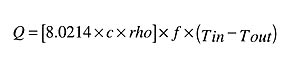
Q = heat output of tube (Btu/hr)
c = specific heat of the fluid (Btu/lb/degrees F)*
d = density of the fluid (lb/ft3)*
C1, C2 = constants based on tube size given in Table 1.
* Fluid properties evaluated at the inlet temperature.
Copper Tube Size C1 Value C2 Value
3/8" -0.236326 0.02286
1/2" -0.238285 0.02665
3/4" -0.237721 0.03695
1" -0.236284 0.04595
1.25" -0.235350 0.05475
1.5" -0.235693 0.06325
2" -0.235996 0.07985
2.5" -0.234942 0.096079
3" -0.234822 0.11189
Equation 2 tracks the continuous drop in fluid temperature along the tube as heat is dissipated. Equation 3 uses the outlet temperature calculated in Equation 2 to determine the total heat output.
Due to the limited significant figures in the values of C1 and C2, this method should only be used when the length of the tube in feet divided by the flow rate in gallons per minute is OVER 20. When the length/flow ratio is under 20, the total heat loss can be accurately determined using Figure 1.
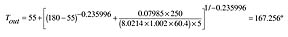
The length in feet divided by the flow rate in gpm is 250/5 = 50, thus the analytical model can be used.
The specific heat and density of 180 degrees F water are approximately 1.002 Btu/lb/degree F, and 60.4 lb/ft3, respectively. Substituting this along with the other data into Equation 2, you will find the results achieved in Equation 2a.
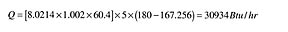
If total heat loss were estimated from Figure 1, the result would be 130 Btu/hr/ft x 250 feet = 32,500 Btu/hr. This is about 5% higher than the result obtained using Equations 2 and 3. Although the difference is small, the analytical model does offer improved accuracy, especially for long piping runs operating at low flow rates.
Manual calculations involving these equations and data are possible, but the overall method begs for software implementation. Equations 2 and 3 and their associated data could be easily integrated into a spreadsheet. The curves in Figure 1 could be described by Equation 1 with the values a and b determined by curve fitting. The software routine could test the length/flow ratio to determine which method to use in finding the overall heat loss.

Insulated Pipe
When insulation is added to the tube, the above model is not valid since it is derived from heat loss data for bare copper tubing.If heat loss data for various insulation/tube combinations were available, and if this data were well described by Equation 1, then new values for the coefficients C1 and C2 could be determined. Equations 2 and 3 could then be used to calculate the total heat output.
A more theoretical approach involves the simultaneous evaluation of convective and radiative heat loss from the surface of the insulation. An iterative procedure is used to find the outside surface temperature of the copper tube at which conduction through the tube equals the total of the convective and radiation heat loss from the outer surface of the insulation.
This procedure is far beyond the realm of manual calculations. It involves repeated calculation of dimensionless parameters such as the Prandtl, Grashof, and Nusselt numbers, as well as non-linear calculations of radiative heat loss. The result of these calculations is an overall heat transfer coefficient that can then be used in an exponential temperature drop model of the insulated tube. A computer-based procedure has been developed by this author for horizontal tubing surrounded by air and covered with one of several types and thicknesses of insulation.(1)
Although the methods described in this article were derived for copper tubing, similar procedures could be used for steel pipe. The ASHRAE Handbook of Fundamentals lists heat loss data for steel pipe in the same format as for copper tubing. New values for the coefficients a and b could be determined by curve fitting Equation 1 to this data. The differential equation shown in Figure 1 could then be integrated using the new values to determine the coefficients C1 and C2. These values could then be used in Equations 2 and 3.
Heat loss from bare copper tubing can be a significant percentage of the total heat output of some distribution systems. Computer models of residential fin-tube baseboard systems indicate that heat loss from bare copper tubing can be in the range of 20% of total circuit heat output. Few designers account for this when sizing baseboard. This heat output provides a safety factor against undersized baseboard if the piping is contained in heated space.
Improved methods for determining piping heat loss, along with software-based implementation of the resulting models, will likely improve the accuracy of future design tools for hydronic heating systems.

