
Figure 1.
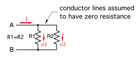
If resistances R1 and R2 are equal, the electrical current through point A will split into equal branch currents passing through R1 and R2. Similar results occur regardless of the number of branches, as long as all branch resistances are equal (e.g., four equal branch resistances will each get 1/4 of the total current flow).
The lines connecting components together in electrical schematics are assumed to have zero resistance. This, of course, is impossible for any real conductor, but when the lines represent very-low-resistance conductors, it’s a reasonable approximation that simplifies circuit analysis.
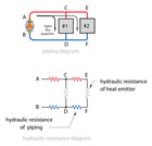
Figure 2.
It’s also apparent that the flow path through heat emitter #2 is longer than that through heat emitter #1. Thus, the flow resistance of path ACEFDB is greater than that of path ACDB. Flows will not divide up equally in such a system. Instead, the branch flows depend on the resistance of the supply and return piping between the branches (e.g., path CE and DF in Figure 2).
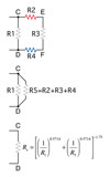
Figure 3.
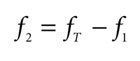
Equation 1.
ƒT = total flow entering node C and leaving node D
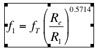
ƒ1 = flow through hydraulic resistance R1
R1 = hydraulic resistance through crossover containing heat emitter #1
Re = equivalent hydraulic resistance determined as shown in Figure 3
Equation 2.
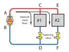
Figure 4.
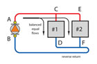
Figure 5.
It’s not wise to assume that every reverse return system will have equal flow proportions through each crossover. Anything that creates a difference in the resistance of the supply or return piping between crossovers will affect these proportions. So would a different type or size of heat emitters in any of the crossovers. A difference in the crossover piping itself (length, type or size) will also change the resistance of that crossover relative to the others and affect flow proportions. For these reasons balancing valves are usually still installed in all the crossovers of reverse return systems, especially large systems with many crossovers or systems that have the potential of being modified over time.
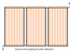
Figure 6.
When Does Reverse Return Make Sense?
Like most concepts in hydronic system design, reverse return has its strengths and limitations. It should not be viewed as one concept that fits all applications.Reverse return subassemblies make sense when two or more identical devices require equal flow proportions from a common supply. An example would be multiple solar collectors, as shown in Figure 6.
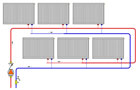
Figure 7.
Reverse return distribution systems make sense when the following conditions are all present:
- The loads are being supplied from a common circulator
- The loads served require the same supply temperature
- The loads served are widely dispersed around the building
- The distribution piping can make a complete loop around the inside of the building starting and ending in the mechanical room.
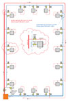
Figure 8.
In systems with relatively short supply and return mains, the designer may elect to use the same pipe size for all mains. This decreases system head loss, which may in turn reduce circulator size. However, it also increases piping cost. A life-cycle cost analysis comparing added hardware cost to reduced operating cost would be the prudent way to evaluate such a tradeoff.
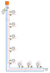
Figure 9.
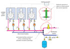
Figure 10.
Controlling DP
Although reverse return systems are closer to “self balancing” than direct return systems, they still cause a fixed speed circulator to experience changes in differential pressure due to changes in flow through the crossovers. Such changes, if uncorrected, can cause flow velocities in active crossovers to increase as valves on other crossovers close. This can lead to flow noise, control valve stem lift and erosion corrosion of copper tubing.One solution is a differential pressure control valve installed across the mains of the system, as shown in Figures 8 and 9. Such valves throttle excess head energy into heat as total system flow drops due to reduced flows in crossovers. Although they accomplish a desired effect (e.g., prevention of excessive differential pressure), they do so in a parasitic manner (e.g., wasting a portion of the head energy of the circulator).
An even better option is a variable-speed distribution circulator programmed to maintain proportional differential pressure control (see “Distribution Efficiency in Hydronic Systems” in June 2006 PME [page 30] for a detailed discussion of this type of differential pressure control). The speed of the circulator automatically adjusts based on the instantaneous flow needs of the distribution system. These “smart” circulators maintain adequate flow while conserving electrical input energy to the pump under partial load conditions. Estimated electrical energy savings from using this approach range from 65% to 80% relative to a fixed-speed wet rotor circulator with PSC motor and equivalent peak performance.
Figure 11.
When It's Not Needed
There are situations where reverse return piping, while possible, does little to improve flow balancing. One example is a multiple boiler system where the boilers are in close proximity and connected to a common header system that has low flow resistance (see Figure 10 on page 31).Because the pressure drop along the boiler header is so low in comparison to the flow resistance through the boiler heat exchanger, there is virtually no difference in the flow resistance through each boiler path and the point of hydraulic separation. A slight variation in circulator performance could make more difference in flow through a given boiler than the boiler’s position along the short low-resistance direct return headers.
Another situation where reverse return is certainly acceptable but not necessarily required is a typical manifold station for floor-heating circuits (see Figure 10). Again, because the pressure drop along the short manifold is extremely low in comparison to the pressure drop along the floor circuit, the use of reverse return piping will have virtually no effect on individual circuit flows. The larger the bore of the manifold relative to the number of circuits it serves, the less effect reverse return piping has. Also keep in mind that the floor circuits may not all be the same length and hence don’t necessarily need equal flow rates.
