Issue: 8/04
In the Jan. 2004 issue of PM Engineer, we discussed the analytical methods involved in designing a hydronic piping circuit. If you didn't read the article, you can find it in the editorial archives at www.pmengineer.com.
The essential steps in designing a hydronic piping circuit were as follows:
- 1. Establish a Target Flow Rate.
2. Determine a tube size.
3. Determine the circuit's system curve.
The January article dealt with methods for series piping circuits. If the designer is working with circuits having parallel branches, the system curve can be determined using the information from the Sept. 2003 PME article, "Determining Flow Rates in Parallel Piping Systems Constructed of Smooth Tubing," also available in the online archives.
Choosing Your Engine
Once the piping system is quantified, the next design task is to select a circulator for the piping system. I like to think of this as matching up an engine with a body and transmission.The circulator needs to supply sufficient head energy to the fluid in the piping system to allow it to achieve and maintain the target flow rate established early in the design process.
The head added by a circulator at a given flow rate is essentially independent of the fluid being pumped. A circulator imparting a head of 20 feet while pumping 60

H = head added by circulator (feet of head)
Delta P = pressure differential across circulator (psi)
D = density of the fluid (lb/ft3)
Curvaceous
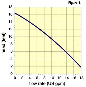
Circulator performance is described by a pump curve, an example of which is shown in Figure 1. Pump curves indicate the head energy imparted to the fluid based on the flow rate through the circulator. The higher the flow rate, the less mechanical energy per pound of fluid (e.g. head) is transferred to the fluid. Manufacturers publish pump curves for all centrifugal pumps they offer. Many now offer software that contains the analytical equivalent of a printed pump curve.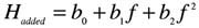
Hadded = head added by circulator (feet of head)
f = flow rate through circulator (gpm)
bo, b1, b2 are constants determined by least square curve fitting
Riding the Curve
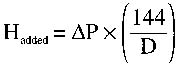
The fact that a circulator always operates along its pump curve makes it possible to find the circuit's flow rate without using a flow meter. What's required is an accurate measurement of the pressure increase across the circulator, and a copy of the circulator's pump curve.The procedure is to convert the pressure increase across the circulator to an associated head using Equation 2. Next, find this head on the vertical axis of the pump curve, and draw a horizontal line over to intersect the pump curve. Finally, draw a vertical line down to the flow rate axis to read the flow.
In Equation 2:
Hadded = head added to fluid by circulator
Delta P = pressure increase measured across circulator (in psi)
D = density of the fluid (in lb/cubic ft)

Striking a Balance
Most things in nature like to be balanced, and head energy is no exception. A closed-loop piping system "wants" to operate where the head energy imparted to the fluid by the circulator exactly balances the head energy dissipated from the fluid by the resistance of the piping system. The point at which this balance occurs is easily found by plotting the pump curve of a "candidate" circulator on the same graph as the system curve for the piping system. The point where the curves cross is called the operating point (Figure 2). It's where head input exactly balances head dissipation. All piping systems quickly settle to this balanced operating condition within a few seconds of the circulator being turned on.Some circulators are designed to produce relatively high heads at lower flow rates. Such circulators are said to have "steep" pump curves. Others produce lower, but relatively stable heads over a wide range of flow rates. Such circulators are said to have "flat" pump curves. These characteristics are fixed by the manufacturer's design of the circulator, in particular the diameter and width of the impeller.
Circulators with steep pump curves are intended for systems having high head losses at modest flow rates. Examples would include series piping circuits containing several components with high flow resistances, earth loop heat exchangers for heat pumps, or radiant floor heating systems using long circuits of small diameter tubing.

Like batteries, circulators can be combined in series or parallel. When two identical circulators are combined in series, the head is doubled at all operating flow rates, as shown in Figure 3a. When two identical circulators are combined in parallel, the flow rate is doubled for each operating head, as shown in Figure 3b.

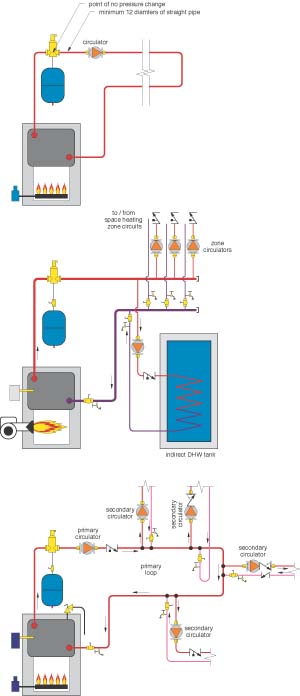
The designer should always include a check valve downstream of each circulator in a parallel combination. These valves prevent reverse flow through a circulator that's off when the other is operating. Also be sure to specify that a minimum of 12 pipe diameters of straight pipe be installed between the discharge port of each circulator and its associated check valve. This segment of pipe reduces turbulence into the check valve and helps prevent rattling of the valve disc.

Circulator Efficiency
Like any device that converts one form of energy to another, a circulator has an associated efficiency.For larger circulators this ratio is usually expressed as the shaft power input divided into the rate of mechanical energy output. Equation 2 can be used to calculate this efficiency, where:
circulator = efficiency of the circulator
f = flow rate through the circulator (gpm)
Delta P = pressure differential measured across the circulator (psi)
1,716 = units conversion factor
hp = horsepower delivered to the circulator shaft by the motor
The efficiency of a pump depends on both the flow rate and differential pressure at which it operates. Efficiency tends to be highest when the operating point lies near the center of the pump curve. It drops off as the operating point moves up or down along the curve. Most pump manufacturers provide plots of pump efficiency on which contour lines representing a given efficiency are drawn.
The efficiency of smaller wet-rotor circulators tends to be expressed as a "wire-to-water" efficiency. This value includes both the mechanical efficiency of the pump as well as the efficiency of the electric motor. Wire-to-water efficiencies, although arguably a better overall indicator of electrical to fluid flow energy conversion, are considerably lower than pump only efficiency. It's common for a small wet-rotor circulator to have a peak wire-to-water efficiency in the range of 20%. Again, this efficiency decreases as the operating point shifts away from the center of the pump curve.

npump & motor = efficiency of the pump and motor assembly as a whole
f = flow rate through circulator (gpm)
Delta P = pressure differential measured across the circulator (psi)
w = input wattage required by the motor (watts)
0.4344 = units conversion factor
The input wattage required by a pump motor is not a fixed value. It depends on where the pump operates on its curve. Therefore, to make use of Equation 3, one needs to know the input wattage at the operating point of the circulator within a given system.
To maintain reasonably high efficiency, circulators should be matched to the system curve of the piping system such that the operating point falls within the middle third of the pump curve.
Location, Location, Location
Circulators should always be located so they are "pumping away" from the point of no pressure change. The latter is where the expansion tank connects to the system.This allows the pressure differential developed across the circulator to add to the static pressure in the system. Higher pressure moves the fluid condition farther away from boiling. It also suppresses the release of dissolved air and helps keep the system operating quietly.
This installation detail should be followed in both single circulator and multiple circulator systems. In the case of primary/secondary piping, it is preferable to locate the secondary circulators so they "pump into" secondary circuits. The primary loop (with attached expansion tank) acts as the pressure reference point (Figure 4).
Cavitation
If the pressure of a fluid entering the circulator impeller drops below the vapor pressure of that fluid, vapor pockets will instantly form within the fluid. One could say that the fluid instantly "boils" as it enters the impeller. As the fluid moves outward across the impeller, its pressure increases and the vapor pockets collapse (or implode). Such implosions create very localized but violent conditions within the fluid that can quickly erode even hardened metal surfaces. This overall process is called cavitation and is to be avoided in all cases.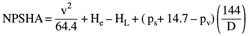
NPSHA = net positive suction head available at the circulator inlet (ft of head)
v = velocity of the liquid in the pipe entering the circulator (ft/sec)
He = distance to the liquid's surface above (+) or below (-) the circulator inlet (ft)
HL = head loss due to viscous friction in any piping components between the liquid surface and the inlet of the circulator (feet of head)
ps = gauge pressure at the surface of the fluid (psig)
pv = vapor pressure of the liquid as it enters the circulator (psi absolute)
The NPSHR is a value determined through testing by the manufacturer. NPSHR generally increases as the flow rate through the pump increases. Most manufacturers can provide a graph showing the NPSHR versus flow rate for the hydronic circulators they offer.
In small and medium scale hydronic systems, good design habits are almost always sufficient to prevent the NPSHA from falling to or below the NPSHR. The following guidelines will help generate the maximum NPSHA for a given system, and thus provide a "safety margin" against the occurrence of cavitation.
- 1. Keep the static pressure on the system as high as practical.
2. Don't operate the system at fluid temperatures higher than necessary. (I suggest limiting boiler outlet temperature to no more than 200
